「アヤメの分類」課題:機械学習のHello World課題
機械学習:分類課題(classification)、教師あり学習
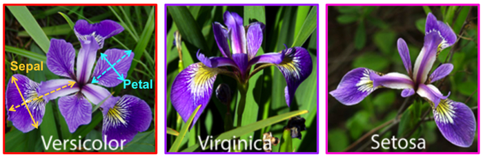
タスク:アヤメのがく片の長さと幅、花弁の長さと幅の4つを特徴量として、アヤメの種類を3つのクラスに分類する。
入力は4次元ベクトル(要素数4の配列:がく片の長さと幅、花弁の長さと幅)、出力は 0(setosa), 1(versicolor), 2(virginica)のいずれかの数
y = f(p, x) 入力 x: 4次元ベクトル,出力 y: 0, 1, 2, p: parameters
教師付き訓練データを利用して,関数 f が正しく出力するように,parametersを調整する。scikit-learn HP: https://scikit-learn.org/stable/
データ構造:NumPy(ndarray), 計算:SciPy,グラフ描画:matplotlib,データ変換:Pandas(DataFrame),scikit-learn のデータセット一覧: https://scikit-learn.org/stable/datasets/toy_dataset.html
【参考】iris(アヤメ)のデータセットをpandasとseabornを使って可視化する https://kenyu-life.com/2019/05/14/iris/
(1)データセットの読込 ---------------
from sklearn.datasets import load_iris  # colabではscikit-learn(sklearn)はインストール済み
iris_dataset = load_iris()  # irisデータセットを読み込む
type(iris_dataset) # typeを確認
sklearn.utils._bunch.Bunch
def __init__(**kwargs)
Container object exposing keys as attributes. Bunch objects are sometimes used as an output for functions and methods. They extend dictionaries by enabling values to be accessed by key, `bunch["value_key"]`, or by an attribute, `bunch.value_key`. Examples -------- >>> from sklearn.utils import Bunch >>> b = Bunch(a=1, b=2) >>> b['b'] 2 >>> b.b 2 >>> b.a = 3 >>> b['a'] 3 >>> b.c = 6 >>> b['c'] 6
Bunchクラスはdictクラスを継承したクラスで、scikit-learnのデータセットはBunchクラスでパッケージングされている。
Bunchオブジェクトではそのキーを属性のように扱って値を取得できる。
iris_dataset.keys() # Bunchクラスはdictを継承しているから、dictの関数keys()も機能する
dict_keys(['data', 'target', 'frame', 'target_names', 'DESCR', 'feature_names', 'filename', 'data_module'])
iris_dataset.DESCR: discription(irisデータセットの説明) ---------------
print(iris_dataset.DESCR)
.. _iris_dataset:

Iris plants dataset
--------------------

**Data Set Characteristics:**

:Number of Instances: 150 (50 in each of three classes)
:Number of Attributes: 4 numeric, predictive attributes and the class
:Attribute Information:
    - sepal length in cm
    - sepal width in cm
    - petal length in cm
    - petal width in cm
    - class:
            - Iris-Setosa
            - Iris-Versicolour
            - Iris-Virginica

:Summary Statistics:

============== ==== ==== ======= ===== ====================
                Min  Max   Mean    SD   Class Correlation
============== ==== ==== ======= ===== ====================
sepal length:   4.3  7.9   5.84   0.83    0.7826
sepal width:    2.0  4.4   3.05   0.43   -0.4194
petal length:   1.0  6.9   3.76   1.76    0.9490  (high!)
petal width:    0.1  2.5   1.20   0.76    0.9565  (high!)
============== ==== ==== ======= ===== ====================

:Missing Attribute Values: None
:Class Distribution: 33.3% for each of 3 classes.
:Creator: R.A. Fisher
:Donor: Michael Marshall (MARSHALL%PLU@io.arc.nasa.gov)
:Date: July, 1988

The famous Iris database, first used by Sir R.A. Fisher. The dataset is taken
from Fisher's paper. Note that it's the same as in R, but not as in the UCI
Machine Learning Repository, which has two wrong data points.

This is perhaps the best known database to be found in the
pattern recognition literature.  Fisher's paper is a classic in the field and
is referenced frequently to this day.  (See Duda & Hart, for example.)  The
data set contains 3 classes of 50 instances each, where each class refers to a
type of iris plant.  One class is linearly separable from the other 2; the
latter are NOT linearly separable from each other.

.. dropdown:: References

  - Fisher, R.A. "The use of multiple measurements in taxonomic problems"
    Annual Eugenics, 7, Part II, 179-188 (1936); also in "Contributions to
    Mathematical Statistics" (John Wiley, NY, 1950).
  - Duda, R.O., & Hart, P.E. (1973) Pattern Classification and Scene Analysis.
    (Q327.D83) John Wiley & Sons.  ISBN 0-471-22361-1.  See page 218.
  - Dasarathy, B.V. (1980) "Nosing Around the Neighborhood: A New System
    Structure and Classification Rule for Recognition in Partially Exposed
    Environments".  IEEE Transactions on Pattern Analysis and Machine
    Intelligence, Vol. PAMI-2, No. 1, 67-71.
  - Gates, G.W. (1972) "The Reduced Nearest Neighbor Rule".  IEEE Transactions
    on Information Theory, May 1972, 431-433.
  - See also: 1988 MLC Proceedings, 54-64.  Cheeseman et al"s AUTOCLASS II
    conceptual clustering system finds 3 classes in the data.
  - Many, many more ...
iris_dataset['target_names']: 分類するクラス名
print(iris_dataset['target_names'])
['setosa' 'versicolor' 'virginica']
iris_dataset.target_names # Bunchオブジェクトはキーを属性のように扱って値を取得できる。
array(['setosa', 'versicolor', 'virginica'], dtype='<U10')
(注)dtypeはNumPyのデータ型表記で '<U10' はUnicode文字列で、
< はリトルエンディアン (複数バイトのデータ量を持つデータを、コンピューターのメモリーに格納したり(あるいは転送したり)する際に、バイトの最下位から順に記録(転送)する方式)
10 は最大文字数を表す
list(iris_dataset.target_names) # arrayはiterableなのでlistにキャストできる
['setosa', 'versicolor', 'virginica']
iris_dataset.feature_names: feature(特徴量): 説明変数 ---------------
データ(特徴量)に情報が無ければ、どのように工夫しても予測はできない!
print(iris_dataset.feature_names) # 特徴量(説明変数):sepal(がく片), petal(花弁)
['sepal length (cm)', 'sepal width (cm)', 'petal length (cm)', 'petal width (cm)']
iris_dataset.data ----------------
type(iris_dataset.data) # scikit-learnのデータ構造は、NumPyのデータ型ndarray:n-dimentinal array)(n次元配列)
numpy.ndarray
len(iris_dataset.data)
150
iris_dataset.data[:10] # 最初の10件を表示
array([[5.1, 3.5, 1.4, 0.2],
       [4.9, 3. , 1.4, 0.2],
       [4.7, 3.2, 1.3, 0.2],
       [4.6, 3.1, 1.5, 0.2],
       [5. , 3.6, 1.4, 0.2],
       [5.4, 3.9, 1.7, 0.4],
       [4.6, 3.4, 1.4, 0.3],
       [5. , 3.4, 1.5, 0.2],
       [4.4, 2.9, 1.4, 0.2],
       [4.9, 3.1, 1.5, 0.1]])
iris_dataset.target: 分類するクラスが数値0, 1, 2(配列target_namesのindex) で表現されている----------------
len(iris_dataset.target) # ここにラベルが格納されている。
150
print(f'{type(iris_dataset.target)=}')
iris_dataset.target  # iris.target_names:['setosa' 'versicolor' 'virginica']
type(iris_dataset.target)=<class 'numpy.ndarray'>
array([0, 0, 0, 0, 0, 0, 0, 0, 0, 0, 0, 0, 0, 0, 0, 0, 0, 0, 0, 0, 0, 0,
       0, 0, 0, 0, 0, 0, 0, 0, 0, 0, 0, 0, 0, 0, 0, 0, 0, 0, 0, 0, 0, 0,
       0, 0, 0, 0, 0, 0, 1, 1, 1, 1, 1, 1, 1, 1, 1, 1, 1, 1, 1, 1, 1, 1,
       1, 1, 1, 1, 1, 1, 1, 1, 1, 1, 1, 1, 1, 1, 1, 1, 1, 1, 1, 1, 1, 1,
       1, 1, 1, 1, 1, 1, 1, 1, 1, 1, 1, 1, 2, 2, 2, 2, 2, 2, 2, 2, 2, 2,
       2, 2, 2, 2, 2, 2, 2, 2, 2, 2, 2, 2, 2, 2, 2, 2, 2, 2, 2, 2, 2, 2,
       2, 2, 2, 2, 2, 2, 2, 2, 2, 2, 2, 2, 2, 2, 2, 2, 2, 2])
# dataとtargetをzipすると、data要素とtarget要素のtupleを要素とするiteratorであるzipオブジェクトとなる
zip_data_target = zip(iris_dataset.data, iris_dataset.target)

print(f'{type(zip_data_target)=}')  # type(zip_data_target)=<class 'zip'>
print(f'{zip_data_target=}')  # zip_data_target=<zip object at 0x780ed115d800>
print(f'{"__iter__" in dir(zip_data_target)=}')  # __iter__メソッドを持つか? True
"""
dir(object)
引数がない場合、現在のローカルスコープにある名前のリストを返す。
引数がある場合、そのオブジェクトの有効な属性のリストを返す。
"""

i = 0
for data, target in zip(iris_dataset.data, iris_dataset.target):
    if( i % 10 == 0):  # 10個置きに表示
        print(f'{data=}, {target=}')
    i += 1
type(zip_data_target)=<class 'zip'>
zip_data_target=<zip object at 0x7dfb47c01800>
"__iter__" in dir(zip_data_target)=True
data=array([5.1, 3.5, 1.4, 0.2]), target=0
data=array([5.4, 3.7, 1.5, 0.2]), target=0
data=array([5.4, 3.4, 1.7, 0.2]), target=0
data=array([4.8, 3.1, 1.6, 0.2]), target=0
data=array([5. , 3.5, 1.3, 0.3]), target=0
data=array([7. , 3.2, 4.7, 1.4]), target=1
data=array([5. , 2. , 3.5, 1. ]), target=1
data=array([5.9, 3.2, 4.8, 1.8]), target=1
data=array([5.5, 2.4, 3.8, 1.1]), target=1
data=array([5.5, 2.6, 4.4, 1.2]), target=1
data=array([6.3, 3.3, 6. , 2.5]), target=2
data=array([6.5, 3.2, 5.1, 2. ]), target=2
data=array([6.9, 3.2, 5.7, 2.3]), target=2
data=array([7.4, 2.8, 6.1, 1.9]), target=2
data=array([6.7, 3.1, 5.6, 2.4]), target=2
(2)データ可視化:データを良く観察する ---------------
これらの特徴量で分類は可能か? データ(特徴量)に情報が無ければ、どのように工夫しても予測はできない!
iris_dataset.DESCR
:Summary Statistics:

============== ==== ==== ======= ===== ====================
                Min  Max   Mean    SD   Class Correlation
============== ==== ==== ======= ===== ====================
sepal length:   4.3  7.9   5.84   0.83    0.7826
sepal width:    2.0  4.4   3.05   0.43   -0.4194
petal length:   1.0  6.9   3.76   1.76    0.9490  (high!)
petal width:    0.1  2.5   1.20   0.76    0.9565  (high!)
============== ==== ==== ======= ===== ====================
petal lengthとpetal widthが分類の良い特徴量、sepal lengthが続く
import matplotlib.pyplot as plt
#petal(花弁)で確認
petal_L = [x[2] for x in iris_dataset.data]
petal_W = [x[3] for x in iris_dataset.data]

fig, ax = plt.subplots()
colors = ['red', 'green', 'blue']  # setosa: red, versicolor: green, virginica: blue
sc = ax.scatter(petal_L,petal_W, c=[colors[i] for i in iris_dataset.target])
ax.set_xlabel("petal_L")
ax.set_ylabel("petal_W")

plt.show()

petal length, petal width: 花弁の長さと幅でプロットすると緑(1) と青(2) の点が少し混在するが、クラスごとに良く分離している。
# sepal(がく片)で確認
sepal_L = [x[0] for x in iris_dataset.data]
sepal_W = [x[1] for x in iris_dataset.data]

fig, ax = plt.subplots()
sc = ax.scatter(sepal_L,sepal_W, c=[colors[i] for i in iris_dataset.target])
ax.set_xlabel("sepal_L")
ax.set_ylabel("sepal_W")

plt.show()

sepla length, sepal width: がく片の長さと幅でプロットするとグループごとの分離は悪い。特に緑(1)と青(2)の点は入り混じっている。
#petal length, sepal length で確認
fig, ax = plt.subplots()
sc = ax.scatter(petal_L,sepal_L, c=[colors[i] for i in iris_dataset.target])
ax.set_xlabel("petal_L")
ax.set_ylabel("sepal_L")

plt.show()

petal length, sepal length:花弁の長さと幅でプロットすると割と良く分離しているが、やはり緑(1) と 青(2) に少し重なりがある。
# 3次元plot
%matplotlib inline
fig, ax = plt.subplots(subplot_kw={"projection": "3d"})
ax.set_xlabel("sepal_L")
ax.set_ylabel("petal_L")
ax.set_zlabel("petal_W")
sc = ax.scatter(sepal_L, petal_L, petal_W, c=[colors[i] for i in iris_dataset.target])

plt.show()


# 視点変更 1
ax.view_init(azim=-30, elev=10)
fig

# 視点変更 2
ax.view_init(azim=-90, elev=10)
fig

# マウスでインタラクティブに回転して観察
# 参考: https://plotly.com/python/3d-scatter-plots/
import plotly.express as px

df = px.data.iris()
fig = px.scatter_3d(df, x='sepal_length', y='petal_length', z='petal_width', color='species', color_discrete_map={'setosa': 'red', 'versicolor': 'green', 'virginica': 'blue'})
fig.show()
Pandasを使えばデータの全てのペアプロットが簡単に得られる -----------------
https://pandas.pydata.org/docs/reference/api/pandas.plotting.scatter_matrix.html
import pandas as pd

iris_df = pd.DataFrame(iris_dataset.data,columns=iris_dataset.feature_names)
grr = pd.plotting.scatter_matrix(iris_df, c=[colors[i] for i in iris_dataset.target], figsize=(15, 15), marker='o', s=50, hist_kwds={'bins': 20}, )
# s=60 散布図のマーカーのサイズ
#'bins':20 散布図行列の対角線上に表示されるヒストグラムのビン(区間)の数を指定

# ヒストグラムを作成
n, bins, patches = plt.hist(iris_df['sepal length (cm)'], bins=20)

# 頻度(絶対度数)を表示
print(n)
[ 4.  5.  7. 16.  9.  5. 13. 14. 10.  6. 10. 16.  7. 11.  4.  2.  4.  1.
  5.  1.]

(3)機械学習 SVM(Suport Vector Machine)
データを訓練データとテストデータに分ける ---------------
全データを学習に利用すると、覚えたことを回答することになり、汎化(generalize)能力があるか分からない。
print(f'{type(iris_dataset.data)=}')
print(f'{type(iris_dataset.target)=}')
type(iris_dataset.data)=<class 'numpy.ndarray'>
type(iris_dataset.target)=<class 'numpy.ndarray'>
データをランダム・シャッフルする
import random
d = list(zip(iris_dataset.data, iris_dataset.target)) ## dataとtargetをzipする
d[40:60] # zipした結果を確認
[(array([5. , 3.5, 1.3, 0.3]), 0),
 (array([4.5, 2.3, 1.3, 0.3]), 0),
 (array([4.4, 3.2, 1.3, 0.2]), 0),
 (array([5. , 3.5, 1.6, 0.6]), 0),
 (array([5.1, 3.8, 1.9, 0.4]), 0),
 (array([4.8, 3. , 1.4, 0.3]), 0),
 (array([5.1, 3.8, 1.6, 0.2]), 0),
 (array([4.6, 3.2, 1.4, 0.2]), 0),
 (array([5.3, 3.7, 1.5, 0.2]), 0),
 (array([5. , 3.3, 1.4, 0.2]), 0),
 (array([7. , 3.2, 4.7, 1.4]), 1),
 (array([6.4, 3.2, 4.5, 1.5]), 1),
 (array([6.9, 3.1, 4.9, 1.5]), 1),
 (array([5.5, 2.3, 4. , 1.3]), 1),
 (array([6.5, 2.8, 4.6, 1.5]), 1),
 (array([5.7, 2.8, 4.5, 1.3]), 1),
 (array([6.3, 3.3, 4.7, 1.6]), 1),
 (array([4.9, 2.4, 3.3, 1. ]), 1),
 (array([6.6, 2.9, 4.6, 1.3]), 1),
 (array([5.2, 2.7, 3.9, 1.4]), 1)]
random.shuffle(d)
d[:10]  # ランダム・シャフル結果を確認
[(array([5.1, 3.8, 1.9, 0.4]), 0),
 (array([4.9, 3. , 1.4, 0.2]), 0),
 (array([6.2, 2.9, 4.3, 1.3]), 1),
 (array([7.7, 2.8, 6.7, 2. ]), 2),
 (array([5.4, 3.4, 1.7, 0.2]), 0),
 (array([4.6, 3.2, 1.4, 0.2]), 0),
 (array([5.5, 2.5, 4. , 1.3]), 1),
 (array([6.3, 3.3, 4.7, 1.6]), 1),
 (array([4.7, 3.2, 1.6, 0.2]), 0),
 (array([5.9, 3. , 4.2, 1.5]), 1)]
train_data = d[:120]    # traning用データとtest用データに分割
test_data = d[120:150]
# 以上の操作をまとめた関数が sklearn.model_selection.train_test_split()
# なお、scikit-learnでは、2次元配列は大文字、1次元配列は小文字を使う習慣があるので、従う。
from sklearn.model_selection import train_test_split as split
X_train, X_test, y_train, y_test = split(iris_dataset.data, iris_dataset.target, train_size=0.8, test_size = 0.2, random_state=10)  # Xは大文字、yは小文字、random_stateで乱数の種を指定するとランダム・シャッフルが再現可能になる
list(zip(X_train, y_train))[:10]  # 確認
[(array([6.6, 2.9, 4.6, 1.3]), 1),
 (array([6.2, 2.9, 4.3, 1.3]), 1),
 (array([7.2, 3. , 5.8, 1.6]), 2),
 (array([5.8, 2.8, 5.1, 2.4]), 2),
 (array([6.3, 2.5, 5. , 1.9]), 2),
 (array([4.6, 3.2, 1.4, 0.2]), 0),
 (array([6.7, 3.3, 5.7, 2.1]), 2),
 (array([6.9, 3.2, 5.7, 2.3]), 2),
 (array([7.7, 2.6, 6.9, 2.3]), 2),
 (array([6.9, 3.1, 5.1, 2.3]), 2)]
学習 ---------------
from sklearn import svm
iris_svm = svm.SVC()  # 機械学習モデルとしてsupport vector machineを選択
iris_svm.fit(X_train, y_train)  # 訓練データで学習
SVC()In a Jupyter environment, please rerun this cell to show the HTML representation or trust the notebook.
On GitHub, the HTML representation is unable to render, please try loading this page with nbviewer.org.
SVC()
予測と評価 ------------------
# 学習済みの識別機iris_svmを利用して,testデータを識別させる
y_pred = iris_svm.predict(X_test)
print(f'{type(y_pred)=}')  # numpy.ndarray
print(f'{y_pred=}')  # 予測値
print(f'{y_test=}')  # 正解(教師データ)

# 正当率: y_pred, y_testともにndarray, ndarrayの比較は要素毎の比較結果のndarrayとなる
print(f'{y_pred == y_test =}')  # 確認: array([ True, True, ・・・, True])

result = list(y_pred == y_test).count(True)/len(y_test)  # 要素毎の比較、count() はlistオブジェクトの関数なので、listへキャスト
print('正当率=', result)

# result < 1. であれば、クラス予測が間違ったデータを表示
if( result < 1.0):
    for i in range(len(y_pred)):
        if y_pred[i] != y_test[i]:
            print(i,' 誤判定:', list(X_test[i]), '予測:', y_pred[i],', 正解', y_test[i] )
type(y_pred)=<class 'numpy.ndarray'>
y_pred=array([1, 2, 0, 1, 0, 1, 2, 1, 0, 1, 1, 2, 1, 0, 0, 2, 1, 0, 0, 0, 2, 2,
       2, 0, 1, 0, 1, 1, 1, 2])
y_test=array([1, 2, 0, 1, 0, 1, 1, 1, 0, 1, 1, 2, 1, 0, 0, 2, 1, 0, 0, 0, 2, 2,
       2, 0, 1, 0, 1, 1, 1, 2])
y_pred == y_test =array([ True,  True,  True,  True,  True,  True, False,  True,  True,
        True,  True,  True,  True,  True,  True,  True,  True,  True,
        True,  True,  True,  True,  True,  True,  True,  True,  True,
        True,  True,  True])
正当率= 0.9666666666666667
6  誤判定: [6.3, 2.5, 4.9, 1.5] 予測: 2 , 正解 1
上記の誤分類はクラス1と2の境界付近で起きている。これは散布図からも了解できる。
# 3次元プロットで誤予測したデータを確認

if( result < 1.0):
    # 分類が間違ったデータ
    X_wrong = []
    y_wrong = []
    y_true = []
    for i in range(len(y_pred)):
        if y_pred[i] != y_test[i]:
            X_wrong.append(X_test[i])
            y_wrong.append(y_pred[i])
            y_true.append(y_test[i])

    for i in range(len(X_wrong)):
        print(f'{X_wrong[i]=}, {y_wrong[i]=}, {y_true[i]=}')


    # 3次元plot
    fig, ax = plt.subplots(subplot_kw={"projection": "3d"})
    ax.set_xlabel("sepal_L")
    ax.set_ylabel("petal_L")
    ax.set_zlabel("petal_W")
    #全データをプロット
    ax.scatter(sepal_L, petal_L, petal_W, c=[colors[i] for i in iris_dataset.target])

    #誤ったデータを上書プロット
    sepal_L_w = [x[0] for x in X_wrong]
    petal_L_w = [x[2] for x in X_wrong]
    petal_W_w = [x[3] for x in X_wrong]
    # 予測が間違ったデータを星型マーク:白, 赤色の枠線 でプロット
    ax.scatter(sepal_L_w, petal_L_w, petal_W_w, marker='*', c="white", edgecolors='red', linewidths=2, s=100)

    plt.show()
X_wrong[i]=array([6.3, 2.5, 4.9, 1.5]), y_wrong[i]=2, y_true[i]=1

# 視点変更 1
ax.view_init(elev=10, azim=-30)
fig

iris_svm オブジェクトのscore()でも、テストセットの正答率を計算できる
iris_svm.score(X_test, y_test)
0.9666666666666667
predict関数の引数はデータの配列
# 誤判定データ[6.3, 2.5, 4.9, 1.5] 判定2,正解1,の近傍でpetal lengthを少し増やしてみる。
x1 = [6.3, 2.5, 4.9, 1.5]
anser = iris_svm.predict([x1])[0]
print(f'x1={x1}: anser={anser} ,{iris_dataset.target_names[anser]}')
x1=[6.3, 2.5, 4.9, 1.5]: anser=2 ,virginica
x2 = x1
x2[3] = x1[3] - 0.1
anser = iris_svm.predict([x2])[0]
print(f'x2={x2}: anser={anser} ,{iris_dataset.target_names[anser]}')
x2=[6.3, 2.5, 4.9, 1.4]: anser=1 ,versicolor
機械学習の分類アルゴリズム:k-最近傍
あるデータに対する予測値は、学習データの中で最も近いデータのラベル(クラス)とする。なお、kはパラメータで最も近いk個の最近傍データの多数決でクラスを決める。
from sklearn.neighbors import KNeighborsClassifier
from sklearn.preprocessing import StandardScaler
scaler = StandardScaler()
# データの規格化
X_train_std = scaler.fit_transform(X_train)
X_test_std = scaler.transform(X_test)

iris_knn = KNeighborsClassifier(n_neighbors=3)
iris_knn.fit(X_train_std, y_train)

iris_knn_score = iris_knn.score(X_test_std, y_test)
print(f'{iris_knn_score=}')
iris_knn_score=0.9666666666666667
(4)学習済みモデル iris_svm を保存、読込
import joblib
joblib.dump(iris_svm, '/content/drive/MyDrive/Colab Notebooks/iris_svm.pkl')  # google driveに保存
['/content/drive/MyDrive/Colab Notebooks/iris_svm.pkl']
iris_svm2 = joblib.load('/content/drive/MyDrive/Colab Notebooks/iris_svm.pkl')
print(f'{iris_svm2.predict(X_test)=}')
iris_svm2.predict(X_test)=array([1, 2, 0, 1, 0, 1, 2, 1, 0, 1, 1, 2, 1, 0, 0, 2, 1, 0, 0, 0, 2, 2,
       2, 0, 1, 0, 1, 1, 1, 2])
まとめ -------------------------------------------------------------------------------
from sklearn.datasets import load_iris
from sklearn.model_selection import train_test_split as split
from sklearn import svm
from sklearn.neighbors import KNeighborsClassifier

iris_dataset = load_iris()  # データセット読込
X_train, X_test, y_train, y_test = split(iris_dataset.data, iris_dataset.target, train_size=0.8, test_size = 0.2, random_state=10)  # 学習用とテスト用に分割

iris_svm = svm.SVC()  # 機械学習モデル選択: support vector machine
iris_svm.fit(X_train, y_train)  # 学習(訓練)

iris_knn = KNeighborsClassifier(n_neighbors=3)  # 機械学習モデル選択: k-最近傍
iris_knn.fit(X_train, y_train)  # 学習(訓練)

iris_svm_score = iris_svm.score(X_test, y_test)  # 評価
print(f'{iris_svm_score=}')

iris_knn_score = iris_knn.score(X_test, y_test)
print(f'{iris_knn_score=}')

x = [4.9, 2.5, 5.0, 1.7]
anser = iris_dataset.target_names[iris_svm.predict([x])][0]  # 予測
print('iris_svm:', x, ':', anser)

anser = iris_dataset.target_names[iris_knn.predict([x])][0]
print('iris_knn:', x, ':', anser)
iris_svm_score=0.9666666666666667
iris_knn_score=0.9666666666666667
iris_svm: [4.9, 2.5, 5.0, 1.7] : virginica
iris_knn: [4.9, 2.5, 5.0, 1.7] : virginica